Neural Model Checking

Abhinandan Pal

The Bug That Should Never Have Happened#

In 1996, Intel shipped millions of Pentium processors with a floating-point division bug, costing about $475 million. In 2018, the Meltdown and Spectre vulnerabilities affected billions of processors worldwide. In 2024, a single software update crashed 8.5 million Windows machines globally, grounding flights and disrupting hospitals.

Here’s the uncomfortable part: testing didn’t catch these before they shipped.

Testing is great at finding bugs, but terrible at proving their absence. You can run a million tests and still miss the one edge case that takes down your system. A 32-bit counter has over 4 billion possible states. For a modern processor, the number of possible states is astronomically large.

This is where model checking comes in.

Model checking doesn’t test your system, it mathematically proves properties about it. Every possible execution. Every edge case. Every race condition. If there’s a bug, model checking can find it. If there isn’t, you get a proof.

This is not theory gathering dust in textbooks. Model checking is how Intel, AMD, and ARM verify processors today. It is how NASA checks spacecraft software. It is how safety-critical components in cars are validated. Three Turing Awards have recognized foundational work in this area (1996, 2007, 2013).

But there’s a problem: model checking is slow. Really slow.

The State Space Explosion Problem#

Imagine you are verifying a simple system with just 10 boolean variables. That is 2^10 = 1,024 states. Add 10 more variables and you are at over a million states. A typical hardware design has hundreds or thousands of variables. The state space grows exponentially, and traditional model checkers can end up exploring an enormous number of states.

For decades, researchers have fought this explosion with clever machinery: binary decision diagrams (BDDs), SAT/SMT solvers, symbolic execution, abstraction, and compositional reasoning. These tools are engineering marvels. But modern designs increasingly involve complex arithmetic (counters, multipliers, floating-point units, bit-level hacks), and those features can make classic representations blow up in size and push even state-of-the-art tools to the edge.

Elevator Pitch for Neural Model Checking#

A lot of verification problems reduce to searching for a function that satisfies a set of mathematical constraints, for example inductive invariants and ranking functions. Neural networks are universal function approximators, so they are a natural fit to represent these objects. The verification constraints become a training objective, with violations showing up as loss.

The catch is that the underlying transition system can have billions of transitions, and naively enforcing proof constraints on all of them is computationally infeasible. However, while the full state space is huge, the “interesting” behavior often concentrates around comparatively few edge cases. In human-written (or LLM-written) code and hardware, individual components tend to be designed to be readable and structured, so the corner cases are usually sparse relative to the full space.

Neural model checking uses a counterexample-guided loop:

1. Sample transitions that are likely to expose edge cases (from simulation, fuzzing, heuristics).
2. Train a neural proof certificate (a neural network representing an invariant, ranking function, etc.) to satisfy the proof conditions on the sampled data. Reaching zero loss means the certificate is correct on the samples.
3. Ask a solver to break it by searching for a counterexample transition where the certificate violates the proof conditions globally. Checking a proposed certificate is typically much easier than finding one from scratch, so this step is comparatively efficient.
4. If the solver finds no counterexample, the certificate is globally valid, and you have a proof for the entire state space. If it finds a counterexample, you add it to the dataset and retrain.

This turns verification into an iterative game: the network proposes a proof, the solver tries to refute it, and any refutation becomes new training data. Over time, the proof certificate converges, and when the solver can no longer break it, you are done.

Experimental Results at a Glance#

Beyond solving more liveness-heavy tasks, the most noticeable win is speed. On the benchmark suite (11 RTL designs, 634 tasks), many instances that push classical model checkers toward the 5-hour timeout finish with neural certificates in seconds to minutes, because the solver is checking a proposed certificate rather than exploring a massive state graph.

Here are the headline speedups reported:

• On proving good things eventually happen: our method is faster, than the fastest tool for each task, on 66% of tasks, with ≥10× speedups on 46%, ≥1000× on 11% and ≥10000× on 4%.
• On proving good things eventually happen and bad things never happen: faster on 61% of tasks, with ≥10× speedups on 52%, ≥100× on 43%, ≥10000× on 27%, and ≥100000× on 6%.
• Compared to our 2024 version: the 2025 approach obtains ≥10× speedups on 88% of liveness tasks, ≥100× on 79%, and ≥1000× on 45%.

This results make implementing verification much more feasible into ones daily workflow which would allow for proveably correct code.

The Model Checking Problem#

Model checking asks:

Does my system M always behave the way my spec P says it should?

• M is the thing you built: a program, hardware circuit, distributed protocol, controller, etc.
• P is a set of hard rules: what you want it to do (and what you forbid it from doing).

A model checker explores all possible executions of M. If it finds even one execution that violates P, it produces a counterexample trace (a step-by-step run showing exactly how things go wrong).

Two Kinds of Properties (And Why Liveness Is Trickier)#

Safety is “find a bug.” If the property is false, a specific step breaks it, so a finite counterexample trace is enough.

Liveness is “rule out procrastination forever.” If the property is false, the system might keep postponing the good event indefinitely. Any finite run cannot disprove liveness because the good thing could happen later. So the checker has to reason about infinite behavior (typically by detecting cycles, ranking functions to reason “can this keep going forever without progress?”).

A classic result says that any “linear-time” property can be viewed as a safety part + a liveness part. Linear Temporal Logic (LTL) is a convenient language to express such properties.

Linear Temporal Logic (LTL): Specifying Behavior Through Time#

Propositional logic talks about one snapshot. LTL talks about an execution through time.

Mini Example#

Suppose a system exposes two 1-bit outputs:

1. q means “done” Liveness: F (q = 1) Read: “Eventually, q becomes 1.”

2. p means “error” Safety: G (p = 0) Read: “At all times, p stays 0.”

An LTL formula is interpreted over an infinite trace, meaning a sequence of states, one per time-step:

(q0=0, p0=0) → (q1=0, p1=0) → (q2=1, p2=0) → (q3=1, p3=0) → ...

This trace satisfies the example property if:

• p is never 1 (no error ever), and
• at some point q becomes 1 (done eventually happens).

Key rule: A system satisfies an LTL property if every infinite trace the system can produce satisfies it.

The Core LTL Operators#

Two common composites:

• G F φ (recurrence) means φ happens infinitely often.
• F G φ (persistence) means eventually φ becomes true forever.

All of these combine normally with Boolean logic (∧ ∨ ¬ →) and predicates/comparisons (= < > ≤ ≥).

A Small Example in Practice#

FG ¬rst  →  (GF (disp = 0) ∧ GF (disp = 1))

Plain English: “Once reset stops happening forever, the controller must still show display 0 infinitely often, and display 1 infinitely often.”

Breakdown:

• F G ¬rst (written as FG ¬rst) means: eventually, reset becomes permanently off.
• G F (disp = 0) means: display 0 keeps coming back, forever.
• G F (disp = 1) means: display 1 keeps coming back, forever.
• The ∧ ensures neither display starves the other.

Model Checking via Emptiness Checking#

1. Modeling a Reactive System#

A reactive program is one that does not terminate, it keeps responding to inputs or updating state forever. We model such a program M using three ingredients:

• State variables X_M: a finite set of variables that fully describe the program’s current state.
• Initial states Init_M: which states the program is allowed to start in.
• Transition relation Update_M(s, s’): which next states s’ are legal after a current state s.

2. Example: A Loop with 16-bit Wraparound#

for (int i = 0; ; i++) ;   // 16-bit signed, so it wraps

Because i is 16-bit signed, it eventually overflows and wraps around. This program has exactly one infinite execution (one infinite trace):

(i = 0) → (i = 1) → (i = 2) → … → (i = 32,767) → (i = -32,768) → … → (i = 0) → …

3. Systems and Properties as Sets of Infinite Traces#

In general, a system can have many possible infinite executions (due to inputs, nondeterminism, concurrency, scheduling, etc.). Let L_M be the set of all infinite traces the system can produce.

Now consider the temporal property:

F (i = 5)   // “eventually, i equals 5”

Let L_P be the set of all infinite traces that satisfy this property (meaning: at some point along the trace, i = 5 occurs).

Model checking asks one clean question:

Is L_M ⊆ L_P? In other words, do all possible behaviors of the system satisfy the specification?

• If yes, the system is correct with respect to P.
• If no, there exists a counterexample trace in L_M ∖ L_P, a real execution the system can follow that violates the property.

4. Turning a “For All” Question into a “There Exists” Question#

Instead of proving that every trace satisfies P, we can show that no traces violate it.

Let L_¬P be the set of traces that violate P (equivalently, the traces that satisfy (¬P)).

Then the system satisfies P exactly when no system trace is a violating trace:

L_M ∩ L_¬ P = ∅

In words: “There is no execution that is both a legal behavior of the system and a violation of the spec.”

This is the key shift: from universal checking to an emptiness question.

5. Büchi Automata: Machines for Infinite Behaviors#

To make this algorithmic, we represent sets of infinite traces using Büchi automata (BA):

• A Büchi automaton reads an infinite sequence of symbols (an infinite trace).
• A run is accepting if it visits designated accepting states infinitely often.

We build automata for two things:

So A_M captures what the program can do, and A_¬ P captures what it means to go wrong.

6. Product Construction = Intersection of Behaviors#

We combine the two automata using a synchronous product:

A_M ∥ ¬ P = A_M ⊗ A_¬ P

This product automaton accepts exactly the traces in:

L_M ∩ L_¬ P

So now the model checking problem becomes:

• If A_M ∥ ¬ P has no accepting run, then the intersection is empty, so every program behavior satisfies P.
• If it does have an accepting run, that run corresponds to a concrete counterexample execution.

We reduced correctness to checking whether the Büchi automaton for “bad behaviors” accepts nothing, meaning whether its language is empty, but doing this directly is expensive because the product automaton A_M ∥ ¬ P can blow up to an exponential number of states. That is why neural model checkers avoid explicitly building or enumerating the full product; instead, they synthesise invariants and ranking functions as neural networks.

Emptiness Checking Using Invariants and Ranking Functions#

The product automaton A_M ∥ ¬ P is the clean theoretical object, but building it explicitly is usually a non-starter. So, in practice, we work with a lightweight, implicit representation of the product and prove it has no accepting run using two proof ingredients: an invariant (what is reachable) and a ranking function (why accepting states cannot repeat forever).

1. Which Product States Are Actually Reachable?#

Instead of enumerating every state of A_M ∥ ¬ P, we keep only the essentials:

• Init_M ∥ ¬ P: the set of initial product states.
• Update_M ∥ ¬ P(s, s’): a relation that says when s’ is a legal successor of s.

An important subtlety:

The transition relation can describe successors from states that are theoretically valid but never actually reachable from the initial states.

If we explicitly constructed the product graph, those unreachable regions would simply never appear during exploration. But when we keep the product implicit, we must account for reachability ourselves.

That is the job of a reachability invariant (Is), a predicate that separates the reachable part of the unrachable:

• (Is = true) means: s is reachable from Init_M ∥ ¬ P.
• (Is = false) means: s is unreachable, so it is irrelevant to the behavior of the system.

To be a valid reachability invariant, I must satisfy two standard conditions:

1. Base: every initial state is marked reachable.

If (s ∈ Init), then (Is) holds.

2. Step: reachability is preserved by transitions. If (Is) holds and (Update(s, s’)) holds, then (Is’) must also hold.

We call this an invariant because once it becomes true along a reachable execution, it stays true for every subsequent state on that execution.

2. Why Accepting States Cannot Repeat Forever#

Reachability alone is not enough. Emptiness for a Büchi automaton is about whether there exists a run that visits accepting states infinitely often. So we need a way to rule that out.

This is where a ranking function comes in.

Think of a function (Rs) that assigns a non-negative integer to each reachable product state:

Rs ∈ {0,1,2,...}

The idea is simple:

• Along any transition between reachable states, the rank never increases.
• Whenever the run visits an accepting state, the rank decreases by some unit.

Intuition: the rank is a counter for accepting states in an infnite run. If accepting states kept appearing forever, the counter would be forced to decrease forever. But a non-negative integer cannot strictly decrease infinitely many times.

So:

• If such a ranking function exists (over reachable states), then no run hits accepting states infinitely often, so the product automaton is empty.
• If there is an accepting run (an infinite run with infinitely many accepting visits), then no such ranking function can exist, because it would imply an infinite descent.

3. The Takeaway#

To prove A_M ∥ ¬ P is empty without constructing it, it is enough to provide:

• an invariant I that correctly describes the reachable part of the product, and
• a ranking function R that strictly drops whenever an accepting state is encountered (on reachable transitions).

Together, they imply: no reachable accepting run exists, hence:

L_M ∩ L_¬ P = ∅   ⇒   L_M ⊆ L_P

Meaning: every execution of M satisfies P.

4. Illustrative Example#

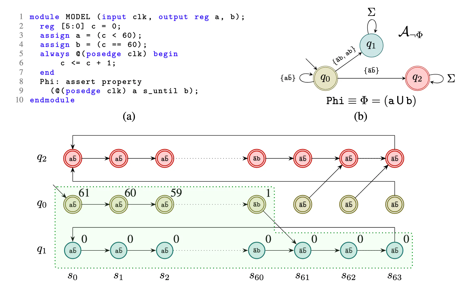Figure 1: End-to-end illustration on a toy example. (a) A 6-bit counter system with signals a and b. (b) Büchi automaton for ¬Φ accepting traces that violate the specification. (c) Product automaton M ∥ A_¬Φ with inductive invariant (dotted region) and ranking values.

Figure 1 illustrates the idea end-to-end on a toy example.

In (a) the “system” is a tiny SystemVerilog module with a 6-bit counter c that increments every clock. We define two Boolean signals: a means “we are still before 60” (c < 60) and b means “we hit 60” (c == 60). The specification is (Φ = a ;U; b), read as: “a must keep holding until b happens, and b must eventually happen.”

In (b) we build the Büchi automaton for (¬ Φ), meaning it accepts exactly the traces that violate the spec. We start in q_0, the “waiting for b” mode. As long as a is true and b is still false, we can keep looping in q_0. If at any point a becomes false before we ever see b (so ¬a ∧ ¬b), that is an immediate violation of the “a holds until b” part, so we move to q_2, an accepting sink that represents “the spec is already broken.” On the other hand, if b does happen, we move to q_1, a non-accepting state where we can stay forever, because once b has occurred, (¬ Φ) can no longer be witnessed. The key liveness point is this: if we were to remain in q_0 forever, that would mean b never happens, so the “eventually b” part fails, and (¬ Φ) should accept. That is why q_0 is also accepting: it flags the “waiting forever” behavior.

In (c) we combine the system and the property-violation automaton into the product M ∥ A_¬ Φ, drawn as a grid of product states (s_i, q_j), meaning “counter value (i) and automaton state q_j,” starting from (s_0, q_0). The dotted region is an inductive invariant I, a set of product states that contains all reachable behavior we care about. Notice that I contains no states paired with q_2, which means “the safety part never breaks” (we never see ¬a ∧ ¬b before b). The small numbers in the grid are the ranking values: within I, the rank never increases, and it strictly drops whenever we are in the accepting “waiting” state q_0. Intuitively, the rank is counting down how many more steps we will keep waiting before b must finally occur. Thus for all infinite trances the accepting states are visited only finitely many time, so no accepting run exists. That is the emptiness proof, and it implies the original system satisfies (Φ).

5. One Function Instead of Two#

You can package both ideas into a single function (Vs) using a threshold (k):

• (Vs > k) means: s is unreachable (so we do not care about it).
• (Vs ≤ k) means: s is reachable, and (Vs) acts as the rank.

This “single certificate” is convenient in practice because you only need to learn or synthesize one object, and it simultaneously answers two questions:

1. Is this state even reachable?
2. If it is reachable, how close are we to the good state?

Enter Neural Networks#

Why Neural Networks?#

Neural networks excel at one specific task that verification constantly needs: representing functions without you having to hand-design them.

That matters because many verification proofs boil down to finding the right function:

• An invariant answers: which states are actually reachable? This is a classification problem (reachable vs unreachable).

• A ranking function answers: are we making progress so we cannot loop forever without the good event? This is a regression problem (assigning a numeric “progress score” to each state).

If we can learn these functions from sample transitions, we can turn “prove this system correct” into “fit a function that satisfies constraints”, and then let a solver do the final, formal check over the entire state space.

Two Flavors of Neural Certificates#

1. Neural Ranking Functions (mainly for Liveness)#

Paper: Neural Model Checking (NeurIPS 2024)

This line of work targets liveness properties, the “something good eventually happens” kind. The neural network represents a ranking function that behaves like a progress meter:

• Along any valid transition, the rank never increases.
• When the execution passes through an accepting state (states that would need to repeat forever to violate liveness), the rank must drop by a fixed margin.

If such a function exists, you have ruled out the possibility of visiting accepting states infinitely often, which is exactly what emptiness checking needs.

Architecture (high level):

• Input: the current system state (for hardware, think register values).
• Network: a small feed-forward model (tiny by ML standards).
• Output: a single number, the “rank”.

Training idea: Training enforces the ranking constraints by penalizing violations.

Loss = max(0, Vs - Vs' + ε · 𝟙_Fs)

Where:

• Vs is the rank at state s
• Vs' is the rank at the next state
• ε is a margin that forces a strict decrease when required
• 𝟙_Fs is 1 if s is accepting, else 0

So the network learns: “Do not go up, and if you are in an accepting state, go down by at least ε.”

After training, the network is quantized (converted into bit vector arithmetic) and then encoded as constraints inside an SMT solver. The solver checks whether the ranking conditions hold for all possible transitions, not just the training set. If the solver says “valid”, you get a formal certificate.

2. Neural Invariants + Ranking in One Certificate (Safety + Liveness)#

Paper: Let a Neural Network Be Your Invariant (NeurIPS 2025)

Real specs rarely come as “pure safety” or “pure liveness”. They usually mix both:

• Safety: “the buffer never overflows”
• Liveness: “every request eventually gets processed”

This approach extends the idea by having one neural network do two jobs at once: mark reachability (safety) and provide a ranking (liveness).

Unified certificate idea:

Vs > k   →   s is unreachable

Vs ≤ k → s is reachable, and Vs acts as its rank

So one scalar output Vs carries both meanings:

• If the value is “large” (above a threshold k), the state is proven irrelevant because it is unreachable.
• If the value is “small” (at most k), the state is reachable, and the value gives the ranking needed to rule out infinite accepting behavior.

Training with constraint solvers (rather than pure gradient descent): A key idea here is to lean more heavily on constraint-solving during training. Compared to standard gradient-based training, this can in practice:

• converge faster in this setting,
• avoid local minima,
• and produce smaller, cleaner networks that are easier for solvers to check.

Note: For the rest of this blog post, we will focus on the NeurIPS 2025 approach, because it gives a single, unified certificate that handles the reality of verification: safety and liveness together, checked with solver-level guarantees.

Learn Check Loop#

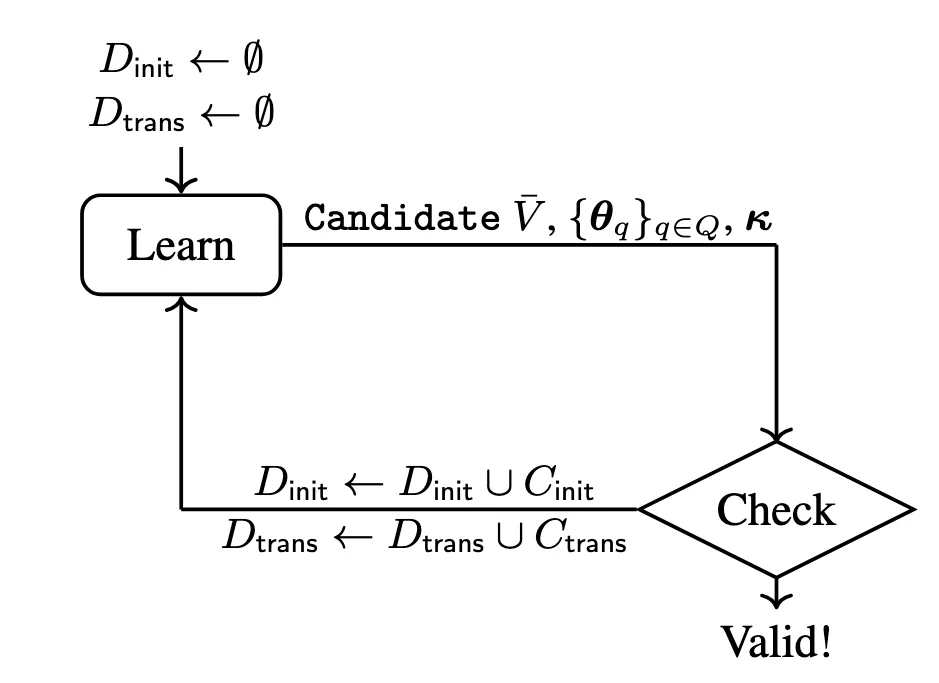Figure 2: The counterexample-guided learning loop. Starting with sampled data, the learn step synthesizes a candidate certificate, then the check step uses an SMT solver to find counterexamples. If counterexamples exist, they’re added to the dataset and the process repeats until the certificate is globally valid.

The figure shows a counterexample-guided loop: we start with no data at all and try to synthesize a candidate certificate anyway. Concretely, we keep two growing datasets, D_init (sampled initial register value) and D_trans sampled one-step transitions of the product (M ∥ A_¬ Φ); the learn step searches for network parameters and a single global threshold (κ) so that the candidate V̄ satisfies the initiation constraint on every sample in D*init, and the “non-increase, strict decrease on accepting” constraint on every sampled transition in D_trans. Then the check step hands this candidate to an SMT solver and asks: “Over the entire state space does there exist any counterexamples to our candidate solution being the true solution” If the solver says SAT, it returns an explicit counterexample (a concrete initial state or a concrete transition), we add it to D_init or D_trans, and the next learn step is forced to fix exactly that edge case; if the solver says UNSAT for both queries, then no remaining counterexamples exist anywhere, so the neural certificate is globally valid and emptiness follows.

The specification automaton is real world cases are tiny, so we can afford to be strategic: instead of running one monolithic counterexample search over the entire product, we run targeted searches per transition of the spec automaton. This naturally gives balanced coverage across the property logic, so every transition in A_¬ Φ gets attention, without relying on hand-tuned sampling heuristics. In Figure 1, the transition from (s_60, q_0) to (s_61, q_1) is just one transition among many, but for that particular property it is the one that matters most. Biasing counterexample search around the spec automaton makes those property-relevant transitions show up early, because the search is explicitly organized around the structure of A_¬ Φ, not around generic exploration of the full state space.

Network Architecture#

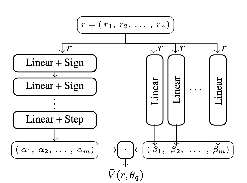Figure 3: Neural certificate architecture. The network takes register values r as input and outputs a score V̄(r,θ_q). The left branch uses sign activations to produce an m-bit mask, while the right branch computes m linear functions. Their dot product yields a piecewise-linear certificate with up to 2^m pieces.

In the figure, the neural certificate takes the current register values (r) (the system state) and outputs a single integer score V̄(r,θ_q). We learn a separate set of parameters θ_q for each specification-automaton state (q). This stays scalable because the spec automaton typically has only a small number of states, even in real world properties. The network is split into two branches. The left branch is a small feed-forward network with sign activations (and a final step) that outputs an (m)-bit mask in 0,1m. Intuitively, this mask “chooses a region” of the input space you can think of it as partitioning the space into up to (2m buckets). The right branch computes (m) simple linear functions of the registers. The final output is their dot product: the mask selects which linear pieces are active, and then adds them up, giving a piecewise-linear scoring function that can represent rich shapes with 2m pieces with just a few neurons. Alongside this, one global threshold exists (κ): values above (κ) are treated as “unreachable” (the invariant side), and values at or below (κ) provide the rank used for the liveness-style argument.

To train this model with a MILP solver, the main idea is to encode the network’s forward computation as linear constraints by adding a small number of helper variables. If we used ReLUs, we would run into a problem: the forward pass repeatedly multiplies weights (variables we are solving for) by activations from previous layer (also variables), which creates products of decision variables, and that turns the optimization into a non-linear problem. The sign activation avoids this. Because a sign output is just (+1) or (-1), multiplying by a weight is either “use the weight” or “use the negated weight”, and that switch can be expressed with standard “implies” constraints in some MILP solvers, or encoded as a set of inequalities (refer to the NeurIPS'25 paper). In other words, the encoding is designed to avoid bilinear (variable-times-variable) terms, which keeps each learning step fast.

MILP learning still does not scale well with huge datasets, but that is where the sampling strategy from the last section matters: we keep the training set small by biasing on the most informative counterexamples and edge cases. That makes the MILP queries practical. It also tends to produce smaller certificates than gradient descent: with gradients, we often needed larger networks to reliably find a satisfying solution, and bigger networks make the final “check” step slower because the solver has more structure to reason about. With MILP, we can often fit the needed constraints with a compact network, which is quicker to verify. Put together, the structured architecture, the MILP-friendly encoding, and the small dataset are what drive the speedups in practice.

Experimental Results#

Setup and what is being measured#

The evaluation uses a benchmark suite of 634 hardware verification tasks derived from 11 SystemVerilog designs, with three spec classes: pure safety, pure liveness, and safety plus liveness. Each tool gets a 5-hour timeout per task, and the experiments run on an AWS m6a.4xlarge machine (16 vCPUs, 64 GB RAM, Ubuntu 24.04). The comparisons include the prior neural baseline NMC’24 and strong symbolic tools nuXmv, rIC3, and ABC/Super-Prove.

Because verification tools are deterministic and must return a provably correct result, the paper reports performance using cactus plots and per-task scatter plots rather than variance bars.

Overall coverage: how many tasks get solved#

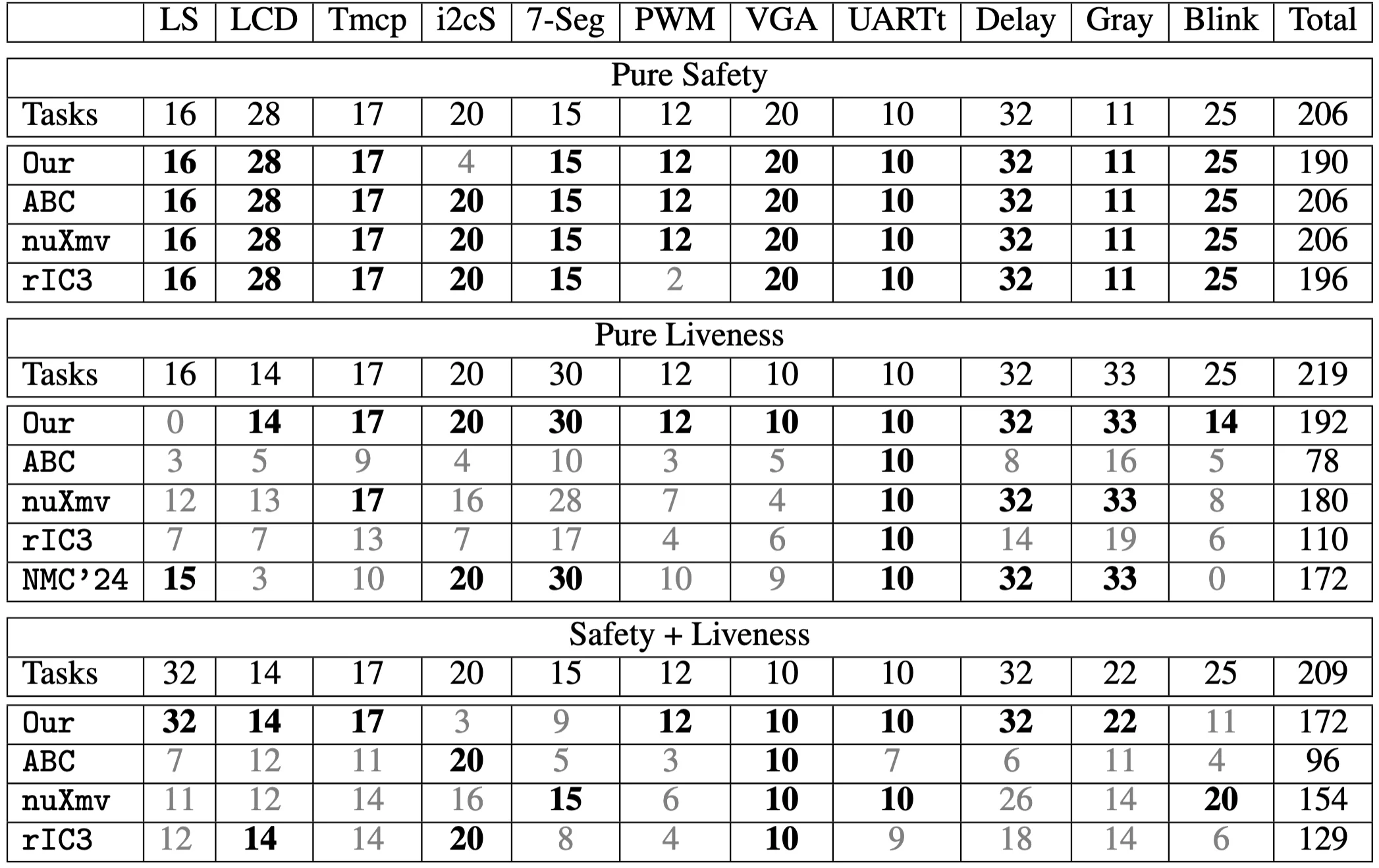Figure 4: Summary table showing the number of tasks solved by each tool across different property classes (pure safety, pure liveness, and safety + liveness).

Figure 4 reports solved tasks by property class.

• Pure safety: 190 of 206 tasks (92%). Symbolic tools solve almost all safety tasks in this suite, so this setting is a high bar.

• Pure liveness: 192 of 219 tasks (88%). The baselines spread out here: nuXmv 82%, NMC’24 79%, rIC3 50%, ABC 36%.

• Safety plus liveness: 172 of 209 tasks (82%). Baselines drop more: nuXmv 74%, rIC3 61%, ABC 46%.

Takeaway: the method stays competitive on safety, and it gains the most once liveness enters, especially when safety and liveness appear together.

Cactus plots#

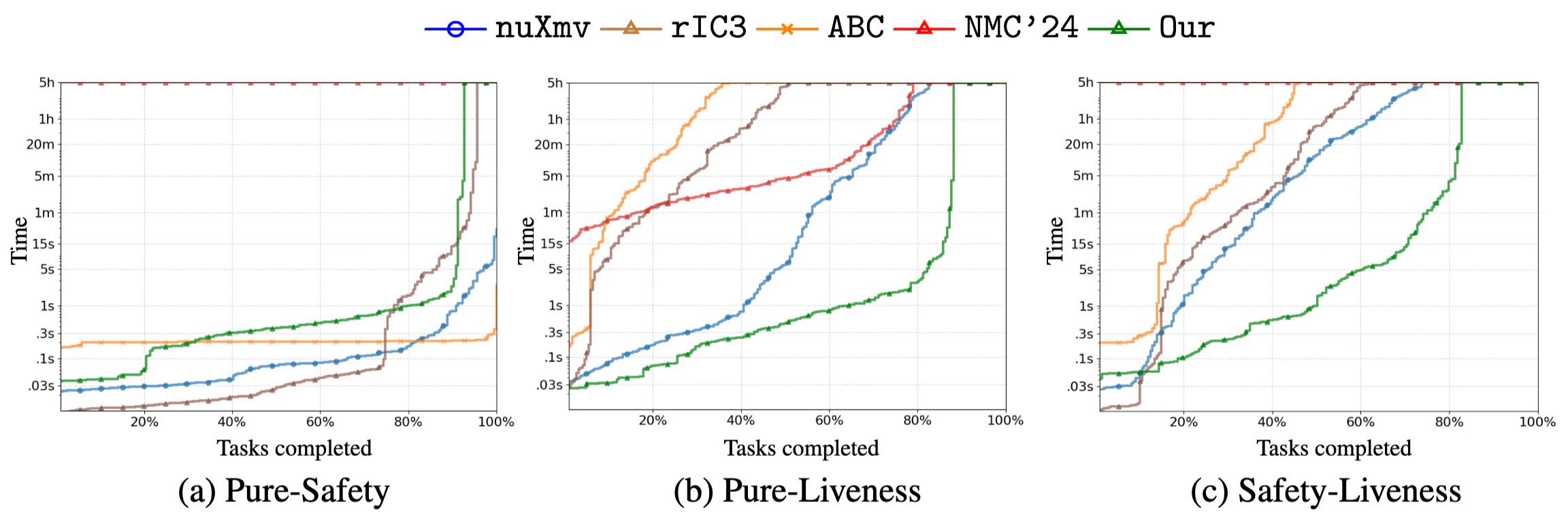Figure 5: Cactus plots comparing neural model checking against classical symbolic model checkers across safety, liveness, and combined verification tasks. Each curve shows the cumulative number of tasks solved as runtime increases.

In these plots, the x-axis is time and the y-axis is how many tasks a tool has finished by that time. Lower and further left is better.

• Pure safety (Figure 5a): performance is close to symbolic tools overall, and the method is faster than nuXmv on 17% of safety tasks, rIC3 on 25%, and ABC on 32%.

• Pure liveness (Figure 5b): the method pulls ahead early. Within 1 second it solves 24% more tasks than nuXmv, 59% more than rIC3, 59% more than ABC, and 64% more than NMC’24. At 1 minute the margins widen to 31%, 68%, 76%, 71%, and after 1 hour they are still 12%, 45%, 59%, 13%. Another useful comparison: tasks that take nuXmv, NMC’24, rIC3, and ABC up to 5 hours per task are completed by this method in under 7s, 3s, 0.6s, and 0.3s per task, respectively.

• Safety plus liveness (Figure 5c): the gap widens further. Within 1 second it completes 31% more tasks than nuXmv, 34% more than rIC3, and 36% more than ABC. After 1 minute the gaps grow to 38%, 43%, 54%, and after 1 hour they remain 20%, 31%, 41%. Benchmarks that exhaust nuXmv, ABC, or rIC3 at 5 hours finish in 56s, 6s, and 0.8s per task with this method. All tools other than this one hit the 5-hour timeout on 18% of the suite.

Scatter plots#

Each point is one task. The x-axis is the fastest competing symbolic tool for that task; the y-axis is this method. Points below the diagonal mean this method is faster. Point size and brightness reflect state-space size.

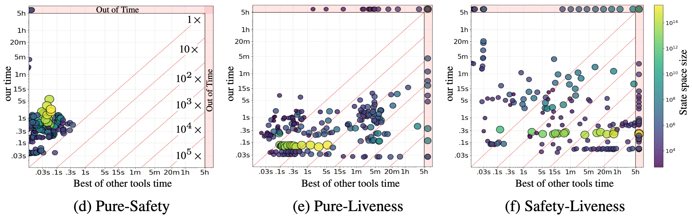Figure 6: Scatter plots showing per-task runtime comparisons. Points below the diagonal indicate tasks where neural model checking is faster than the best competing symbolic tool.

• Pure safety (Figure 6a): On 80% of tasks, both the symbolic winner and this method finish within 1 second.

• Pure liveness (Figure 6b): faster on 66% of tasks; at least 10× faster on 46%; 100× on 29%; 1,000× on 11%; 10,000× on 4%; 100,000× on 1%. Against NMC’24 specifically, speedups of at least 10× appear on 88% of tasks, and at least 100× on 79%.

• Safety plus liveness (Figure 6c): faster on 61% of tasks; at least 10× faster on 52%; 100× on 43%; 1,000× on 36%; 10,000× on 27%; 100,000× on 6%.

Ablations Study#

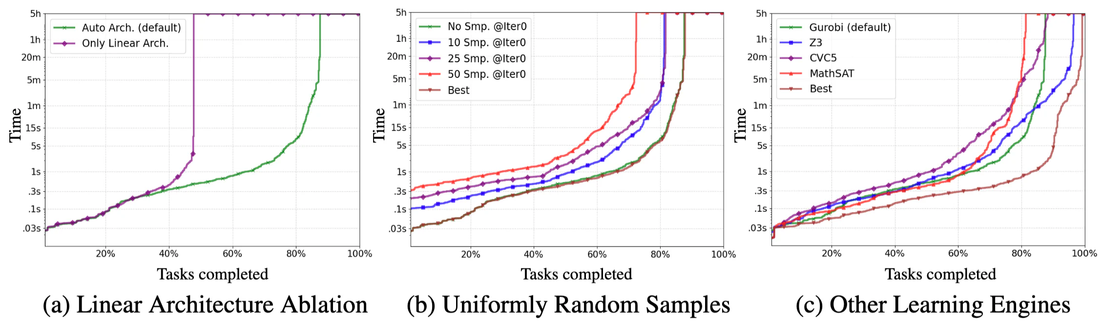Figure 7: Ablation studies showing the impact of neural expressivity, counterexample-guided learning, and different solver backends on overall performance.

Expressivity (Figure 7a)#

The default configuration starts with a linear certificate per spec automata state and escalates only if needed. The linear-only ablation solves 48% of tasks within 9 seconds per task and then stalls; the default reaches 87% overall. This shows that many instances need the extra expressivity of the neural certificate.

Random data vs only counterexamples (Figure 7b)#

The loop starts with empty datasets and grows them using counterexamples. Adding 10, 25, or 50 uniformly random samples does not help much; the default curve is nearly indistinguishable from the per-instance best setting. The solver-guided counterexamples already focus training on the cases that matter.

Learning engine (Figure 7c)#

The paper swaps the learn phase between Gurobi (MILP) and SMT solvers. Within the 5-hour timeout, MathSAT completes 81% of tasks, Gurobi 87%, CVC5 88%, and Z3 96%. On solved instances, Gurobi runs about 7× faster than Z3 on average, but it fails to return a result in 13% of cases due to issues like segmentation faults, infeasibility under the chosen hyperparameters, or numeric mismatches.

Quick Recap#

The key insight: proving system correctness comes down to finding the right mathematical function.

1. Correctness proofs need certificates: To prove a system is correct, you need to find a mathematical function (like a ranking function for liveness or an invariant for safety) that satisfies certain rules.

2. Rules must hold everywhere: These functions must follow specific constraints across the entire state space—not just for some examples.

3. Neural networks are function approximators: This is what they do best—learn complex functions from data.

4. Generate random executions: Run your system randomly (like running test) to collect sample transitions.

5. Train the network as your certificate: Treat the mathematical rules as your loss function. The network learns to be a ranking function or invariant by minimizing violations of these rules.

6. Zero loss = rules satisfied on samples: When training converges (loss = 0), the network satisfies all the rules on your training data.

7. Verify with SMT solvers: Use a SAT/SMT solver to formally check whether the learned function satisfies the rules for every possible state—not just the samples.

The result? If the solver says “yes,” you have a mathematically sound proof of correctness. If it says “no,” it gives you a counterexample—a specific transition where the rules break. Add that to your training data and retrain.

The Future: Where Do We Go From Here?#

Neural model checking is still early, but it already hints at a different workflow for verification: learning proposes a proof candidate, and solvers certify it. Some promising directions:

1. Richer Neural Architectures#

• Graph neural networks to exploit structure in circuits, control-flow graphs, and protocols.
• Hybrid models that explicitly combine symbolic features obtained through static analysis with learned components.

2. Solvers Designed for the Loop#

Today we use one engine to learn and a different one to check, and they share little information. In neural model checking, verification is not a single SAT/UNSAT question. It is an iterative game: propose a certificate, find a counterexample, update dataset, repeat. Solvers built specifically for this workflow could be much faster and more stable than general-purpose tools.

3. Transfer Learning#

Many designs reuse the same patterns (counters, arbiters, FIFOs, pipelines). A natural question is whether we can pre-train on common motifs and fine-tune quickly for a new design or property, possibly even learning which certificate architectures work best for which kinds of systems.

4. Beyond Hardware#

The same certificate-based idea applies broadly:

• Software verification (invariants and termination arguments).
• Cyber-physical systems (controllers for robots, drones, cars).
• Distributed systems (protocols, fairness, and consensus).

5. Theoratical Results#

We also want sharper theoretical understanding: when and why particular certificate families are expressive enough, how to design architectures that match proof structure, and how static analysis can reduce the learning burden by providing strong features, abstractions, or candidate templates.

Further Reading#

Papers

• Neural Model Checking (NeurIPS 2024): https://www.amazon.science/publications/neural-model-checking
• Let a Neural Network Be Your Invariant (NeurIPS 2025): https://www.amazon.science/publications/let-a-neural-network-be-your-invariant

Acknowledgments#

This work was supported by the Advanced Research + Invention Agency (ARIA) under the Safeguarded AI programme.